Statistical Process Control (SPC) is a methodology for monitoring, controlling, and improving a process through statistical analysis of its outputs.

It’s widely used in manufacturing, service operations, and nearly any repeatable process where consistency and quality matter

Think of SPC as your process’s health monitor—constantly collecting data like part sizes, cycle times, or defect counts and plotting them on charts.

By comparing real‑time results to statistically calculated “normal” ranges (usually the mean plus or minus three standard deviations), SPC helps you tell everyday wiggles apart from serious hiccups.

In practise, operators will regularly jot down sample data and keep a quick eye on the control charts to spot anything unusual.

Quality engineers analysis this data, looking for patterns, diving into out-of-control signals and running capability studies to see how well the process is performing.

These insights can be utilised to focus on the right improvement projects and assess if fixes and alterations to a process, actually work.

Instead of reacting to problems after the fact, SPC helps everyone stay ahead of the curve by turning raw data into clear, actionable signals.

SPC are essential for testing the feasibility of processes in the initial prototype stage of a design. By carrying out this nature of analysis you can understand your process capabilities, allowing for data driven decision-making when carrying out FMEA.

By carrying out effective sample measurements within these processes, you can assess whether your results are aligning with the specifications required. Allowing to learn were discrepancies within a more controlled and visible testing environment.

How SPC can help your organisation.

Detecting Problems Early

By continuously monitoring data in real time, SPC alerts you to special‑cause variation before it turns into a large batch of defects or downtime. Early detection means quicker investigation and corrective action.

Driving Continuous Improvement

SPC provides objective, numerical evidence of how changes—new equipment, adjusted procedures, training—affect process stability and capability. Teams can quantitatively assess improvements over time.

Reducing Waste & Costs

Limiting variation means fewer defects, less rework, lower scrap rates, and more predictable throughput. That directly cuts costs and improves overall efficiency.

Meeting Regulatory & Customer Requirements

Many industries (automotive, aerospace, pharmaceuticals, food) require documented quality systems. SPC charts and capability studies are often a core part of compliance with standards like ISO 9001, IATF 16949, or FDA regulations.

Supporting Decision‑Making

Instead of reacting to “eyeballed” or batch‑level quality checks, managers use SPC’s statistical signals to make informed decisions—e.g., when to perform maintenance, adjust process settings, or order new tooling.

Let’s use an example SPC/Process Capability Study, to better understand the parameters and techniques used.

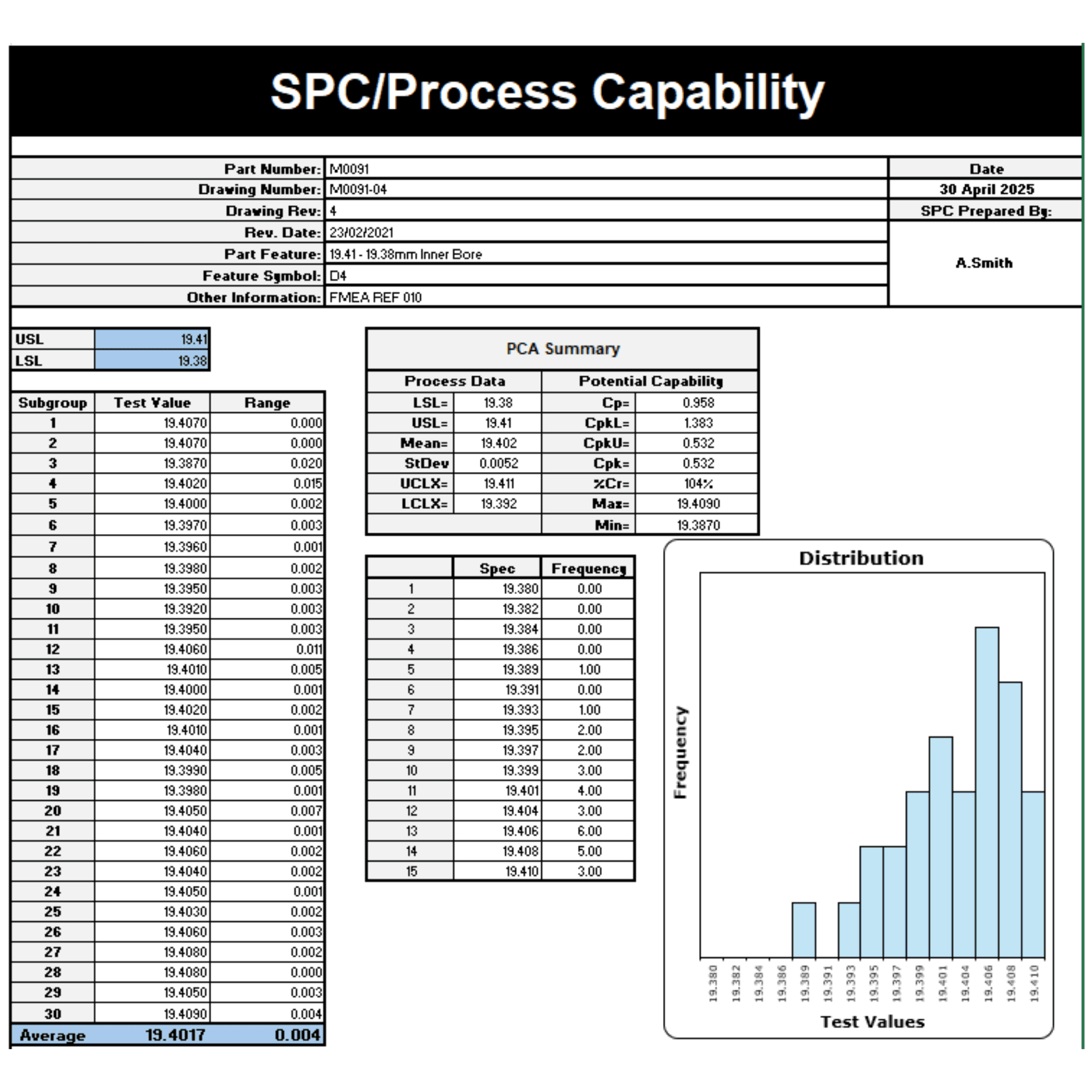
What are these value and what do they mean?

🔹 Specification Limits (USL and LSL)

Your specification limit are the boundaries your measurements are allowed to fall within.

They are typically fixed by design and represent what’s acceptable to customer specifications and engineering functionality of the product.

• USL = Upper Spec Limit

• LSL = Lower Spec Limit

As the "pass/fail" limits, these tolerances are the black and white of any capability study. Any data point outside these parameters result in a failed part.

Process capability aside, these are the bread and butter of any process study. In the main, if parts are correct to specification they conform to their indented purpose.

However, if this is the only parameter you account for within your measurements and process validation, you leave yourself exposed to ignores how consistent a process is.

Parts may be in spec now, but high variation or drift can quickly lead to defects. This further interrogation and insight into our data is were SPC comes in.

🔹 Mean (Average)

Your mean is your central value — a simple average of all your data points.

It shows where your process is centred. Within SPC, if your mean is drifting toward a spec limit and not within your ‘nominal’ mean tolerance, your process is at risk of going out of spec.

Your mean should fall near the midpoint between USL and LSL using our example, our USL = 19.41 and our LSL = 19.38, meaning our nominal mean value equals 19.395.

By calculating our mean we get a figure of 19.402. This suggests our higher than nominal spec and slightly at risk of going above our top limit spec.

🔹 Standard Deviation (σ or s)

Standard Deviation or StDev, is a measurement of how much your data spreads out and varies from the nominal mean.

The smaller the standard deviation, the more consistent and repeatable your process is, as this describes a reduced amount of variation from your average figure.

With our SPC, the StDev is 0.0052 which describes our data set is +/-0.0052 from the nominal mean on average.

Even though the standard deviation is low, our tolerances is very tight. Resulting in the process being slightly sporadic to be consistently within spec long-term.

Our Standard Deviation value will be taken into account for other key metrics within our capability study.

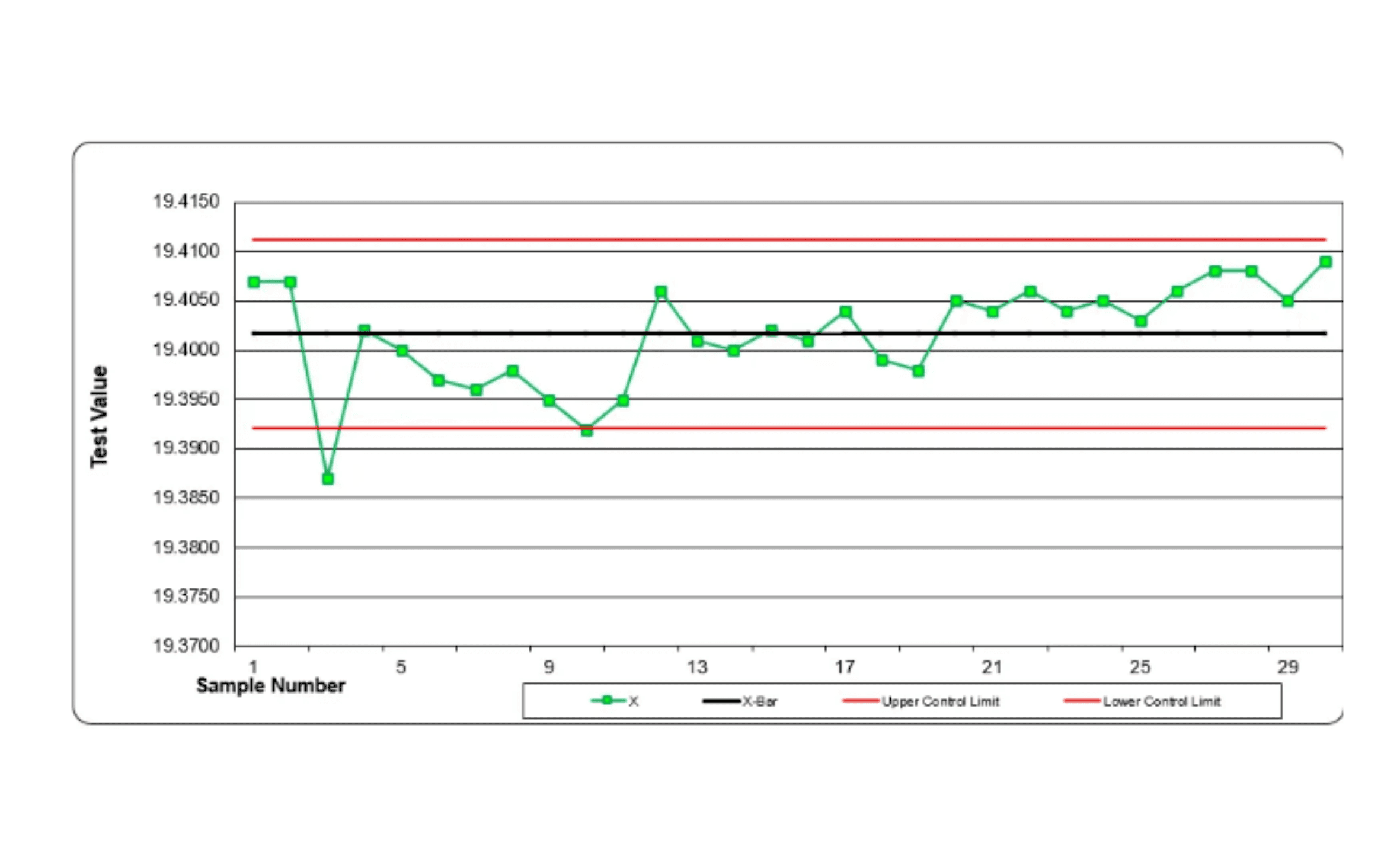
🔹 UCLX / LCLX (Upper & Lower Control Limits – X̄ Chart)

UCLX and LCLX are the control limits that tell you where your process average is expected to stay, as long as everything is running normally.

They’re not about what's acceptable (that’s what spec limits are for), but about what's statistically expected based on how your process normally behaves.

Imagine watching a heart monitor, the lines go up and down, but you know what’s normal. UCLX and LCLX are like that “normal range.”

They’re calculated using your process average and the spread of the data (usually 3 standard deviations above and below the mean).

If a result goes outside these limits, it’s a sign something unusual is happening, like a shift in the process, a faulty tool, or external noise.

Our UCLX of 19.411 and LCLX of 19.392 suggests that our expected range is shifted toward the upper range of our spec (19.41 - 19.38).

It’s not necessarily a defect, but it is a red flag that the process may need attention. These control limits helping prevent problems early, before bad parts are made.

🔹 Cp (Process Capability - Potential)

Cp or Process Capability is a defining metric that measures the robustness of your process.

It does this by measuring how capable your process could be if centered perfectly.

Think of a darts player, he may not be throwing darts in the right place but his grouping of the darts are very close.

Cp proves how consistent your results are within the range of each other.

It does this by comparing the width of your spec limits to the width of your process spread (6σ).

The higher the better, typically a measurement of > 1.33 is good and >1.67 being great.

Our Cp of 0.958 tell us our process not robust enough as the process spread is too high.

🔹 Cpk (Process Capability - Actual)

Cpk considers if your process is centered or not.

Working in reserve to your Cp, Cpk shows actual capability through the spread of you data.

A low Cpk often means you're hugging one spec limit, identifying for any shift or bias.

Cpk alone will only show how centred your results are, this means even if very poor results with a wide spread, you may still find consistency of error.

Cpk is extremely insight because it demonstrates the consistency and robustness for your process even if it out of specification.

With an out of spec but consistent process you are most likely on the right track capability wise, meaning it will be easier to find problems and solve problems systematically.

The standard of Cpk is the same as Cp, with >1.33 being an acceptable standard. Our Cpk of 0.532 explains an offset spread, a fair lack of consistency and a pattern of hugging one spec limit.

🔹 CpkU & CpkL

CpkU and CpkL are two versions of Cpk that look at each end of your spec limits separately. While Cpk gives you the overall capability of your process, CpkU and CpkL break it down.

CpkU checks how close your car is drifting toward the upper side of your tolerances limit (USL). With CpkL, checking how close you are to the lower side of your tolerances limit (LSL).

Your process might be tight and consistent — but if it’s not centered, you’re still at risk of crashing into one side.

They factor in both process variation (σ) and your processes specification limits, meaning is a practical solution that works with your physical measurements over concept.

The lower of the two becomes your overall Cpk, because it represents the weakest point.

Identically to Cp, values over 1.33 are considered capable. Over 1.67 is excellent. Anything under 1.00 means your process is too close to a spec limit and over a large production run, likely producing defects.

Our CpkL is 1.383 which is good however our CpkU of 0.532 further confirms our process is evidentially to close to the upper specification limit.

🔹 %Cr (Capability Ratio Percentage)

%Cr stands for Capability Ratio. It tells you how much of the allowed tolerance your process is actually using.

It compares the spread of your process (6σ) to the width between your upper and lower spec limits.

Think of it like packing a suitcase. If your clothes (process spread) fit easily in the suitcase (spec limits), all good. If you're stuffing it too full, that’s a high %Cr, and things might pop out.

Effectively, a lower %Cr means your process is tight and well within limits. Meanwhile, a higher %Cr means you're pushing too close to the edges.

%Cr helps you see how tight or loose your process is, and whether it's at risk of going out of spec, even if it's currently in control.

General guidance:

• < 50% = Excellent (lots of room to move)

• < 75% = Acceptable

• 100% = Not good — your process spread is wider than your spec limits

Our %Cr of 104% means the variation is wider than the allowed tolerance range, using more space than is acceptable for a robust process.

This indicates the process is not capable, even if it's centred, some results over a longer production run, will fall outside the spec limits.

Summary

Without data, any decision-making you carry out within your organisation is blind. SPC goes beyond charts and stats., it’s a hands-on tool that helps you stay one step ahead.

Instead of scrambling after issues, you catch them before they spiral whether it’s a worn tool, drifting material quality or just everyday variation. It gives you the proof you need when tweaking processes and helps answer the big question: is this actually working?

Whether you're experimenting with a prototype or running full production, SPC keeps things consistent, cost-effective and within spec. And with industry standards to meet, it gives managers and teams the clarity to make smarter faster decisions without the guesswork.

An SPC is only as good as the data that is inputted. Make sure measurement systems are robust and techniques such as: Gauge R&R and Measurement System Analysis, are conducted before any measurements are recorded.

When adjusting a process with your SPC analysis, ensure the data you collected is controlled in order to ensure a fair test is carried out and no changes are made within the same set of test data.

When adjustments are made to a process, they need to be documented. This gives you intel on what was changed, how it was changed and will allow you to account how specific modifications affected your process and it’s test results.